Estimate ATTs from models fits

apm_est() computes the ATTs from the models previously fit by apm_pre(), choosing the optimal one by minimizing the largest absolute average prediction error across validation times. Optionally, this process can be simulated to arrive at a distribution of ATTs that accounts for the uncertainty in selecting the optimal model. plot() plots the resulting ATT(s).

Usage

apm_est(
  fits,
  post_time,
  M = 0,
  R = 1000L,
  all_models = FALSE,
  cl = NULL,
  verbose = TRUE,
  ...
)

# S3 method for class 'apm_est'
summary(object, level = 0.95, M = NULL, ...)

# S3 method for class 'apm_est'
plot(x, label = TRUE, size.weights = TRUE, ...)

Arguments

fits: an apm_pre_fits object; the output of a call to apm_pre().
post_time: the value of the time variable considered post-treatment, for which the ATT is to be estimated.
M: the sensitivity parameter for set identification. For apm_est(), the default is 0, i.e., under point identification. For summary(), this can be set to one or more positive values to produce uncertainty bounds for each value. Only allowed when not set to 0 in the call to apm_est(). See Details.
R: the number of bootstrap iterations used to compute the sampling variance of the ATT. Default is 1000. More is better but takes longer.
all_models: logical; whether to compute ATTs for all models (TRUE) or just those with BMA weights greater than 0 (FALSE, default). This will not effect the final estimates but leaving as FALSE can speed up computation when some models have BMA weights of 0.
cl: a cluster object created by parallel::makeCluster(), an integer to indicate number of child-processes (ignored on Windows) for parallel evaluations, or "future" to use a future backend. NULL (default) refers to sequential evaluation. See fwb::fwb() for details and issues related to replicability.
verbose: logical; whether to print information about the progress of the estimation, including a progress bar. Default is TRUE.
...: other arguments passed to fwb::fwb().
level: the desired confidence level. Set to 0 to ignore sampling variation in computing the interval bounds. Default is .95.
x, object: an apm_est object; the output of a call to apm_est().
label: logical; whether to label the ATT estimates. Requires ggrepel to be installed. Default is TRUE.
size.weights: logicsl; whether to size the points based on their BMA weights. Default is TRUE.

Value

apm_est() returns an apm_est object, which contains the ATT estimates and their variance estimates. The following components are included:

BMA_att: the BMA-weighted ATT
atts: a 1-column matrix containing the ATT estimates from each model (when all_models = FALSE, only models with positive BMA weights are included)
BMA_var: the total variance estimate for the BMA-weighted ATT incorporating the variance due to sampling and due to model selection
BMA_var_b: the bootstrap-based component of the variance estimate for the BMA-weighted ATT due to sampling
BMA_var_m: the component of the variance estimate for the BMA-weighted ATT due to model selection
M: the value of the sensitivity parameter M
post_time: the value supplied to post_time
observed_means: a matrix of the observed outcome means at each pre-treatment validation period
pred_errors: an array containing the average prediction errors for each model and each pre-treatment validation period
pred_error_diffs: a matrix containing the difference in average prediction errors between groups for each model and each pre-treatment validation period
BMA_weights: the BMA weights computed by apm_pre() (when all_models = FALSE, only positive BMA weights are included)
boot_out: an fwb object containing the bootstrap results

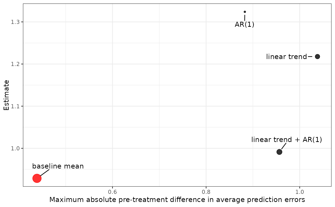
plot() returns a ggplot object displaying the ATT for each model plotted against the maximum absolute difference in average prediction errors for that model. The model with the lowest maximum absolute difference in average prediction errors is displayed in red.

summary() produces a table with the BMA-weighted ATT, it's estimated standard error, and confidence interval limits. When M is greater than 0, additional rows for each value of M are included with the lower and upper bound. When level is greater than 0, these bounds include the uncertainty due to sampling and model selection; otherwise, they correspond to the set identification bounds for the ATT.

Details

apm_est() estimates the ATT from each model and combines them to form the BMA-weighted estimate of the ATT. Uncertainty for the BMA-weighted ATT is computed by combining two variance components, one that account for sampling and another that accounts for model selection. The component due to sampling is computed by bootstrapping the process of fitting the outcome model for the post-treatment outcome identified by post_time and computing the difference between the observed outcome mean difference and the model-predicted outcome mean difference. The fractional weighted bootstrap as implemented in fwb::fwb() is used to ensure no units are dropped from the analysis. In each bootstrap sample, the BMA-weighted ATT estimate is computed as the weighted average of the ATTs computed from the models using the fixed BMA weights computed by apm_pre(), and the variance is computed as the empirical variance over the bootstrapped estimates. The variance component due to model selection is computed as the BMA-weighted variance of the original ATTs.

When M is greater than 0, bounds for set identification and their uncertainty are additionally computed. This involves bootstrapping the fitting of the pre-period models along with post-treatment models on order to compute the maximum absolute difference in average prediction errors for each model across validation periods. Each bootstrap sample produces a margin of error for each model computed as \(M \times \delta_m\) where \(\delta_m\) is the maximum absolute difference in average prediction errors for model \(m\). Upper and lower bounds for the set-identified BMA-weighted ATT are computed as \(\text{ATT}_m \pm M \times \delta_m\). The same procedure as above is then used to compute the variance of these bounds.

summary() displays the BMA-weighted ATT estimate, its standard error, and Wald confidence intervals. When M is greater than 0, bounds for the set-identified ATT are displayed in the confidence interval bound columns. The lower bound is computed as \(\text{LB} - \sigma_{LB}Z_{l}\) and the upper bound as \(\text{UB} + \sigma_{UB}Z_{l}\), where \(\text{LB}\) and \(\text{UB}\) are the lower and upper bounds, \(\sigma_{LB}\) and \(\sigma_{UB}\) are their variances accounting for sampling and model selection, and \(Z_{l}\) is the critical Z-statistic for confidence level \(l\). To display the set-identification bounds themselves, one should set level = 0.

Examples

data("ptpdata")

# Combination of 4 models: 2 time trends, 2 lags
models <- apm_mod(list(crude_rate ~ 1),
                  lag = 0:1,
                  time_trend = 0:1)
models
#> - Model 1: baseline mean
#> crude_rate ~ 1
#> family: gaussian(link = "identity")
#> outcome lag: none
#> outcome diff: none
#> log outcome: no
#> time trend: none
#> unit fixed effects: no
#> 
#> - Model 2: AR(1)
#> crude_rate ~ 1
#> family: gaussian(link = "identity")
#> outcome lag: 1
#> outcome diff: none
#> log outcome: no
#> time trend: none
#> unit fixed effects: no
#> 
#> - Model 3: linear trend
#> crude_rate ~ 1
#> family: gaussian(link = "identity")
#> outcome lag: none
#> outcome diff: none
#> log outcome: no
#> time trend: linear
#> unit fixed effects: no
#> 
#> - Model 4: linear trend + AR(1)
#> crude_rate ~ 1
#> family: gaussian(link = "identity")
#> outcome lag: 1
#> outcome diff: none
#> log outcome: no
#> time trend: linear
#> unit fixed effects: no

# Fit the models to data; unit_var must be supplied for
# fixed effects
fits <- apm_pre(models,
                data = ptpdata,
                group_var = "group",
                time_var = "year",
                val_times = 2004:2007,
                unit_var = "state",
                nsim = 100,
                verbose = FALSE)

est <- apm_est(fits,
               post_time = 2008,
               M = 1,
               R = 20,
               verbose = FALSE)

est
#> An `apm_est` object
#> 
#>  - grouping variable: group
#>  - unit variable: state
#>  - time variable: year
#>    - validation times: 
#>    - post-treatment time: 2008
#>  - sensitivity parameter (M): 1
#>  - bootstrap replications: 20
#> 
#> Use `summary()` or `plot()` to examine estimates and uncertainty bounds.

# ATT estimate and bounds for M = 1
summary(est)
#>       Estimate Std. Error  CI low CI high z_value Pr(>|z|)    
#> ATT     1.0305     0.1745  0.6884  1.3726   5.904 3.55e-09 ***
#> M = 1        .          . -0.1331  2.5279       .        .    
#> ---
#> Signif. codes:  0 ‘***’ 0.001 ‘**’ 0.01 ‘*’ 0.05 ‘.’ 0.1 ‘ ’ 1

# Bounds for other values of M
summary(est, M = c(.5, 1, 1.5, 2))
#>         Estimate Std. Error  CI low CI high z_value Pr(>|z|)    
#> ATT       1.0305     0.1745  0.6884  1.3730   5.904 3.55e-09 ***
#> M = 0.5        .          .  0.3839  1.9270       .        .    
#> M = 1          .          . -0.1331  2.5280       .        .    
#> M = 1.5        .          . -0.7242  3.1420       .        .    
#> M = 2          .          . -1.3353  3.7620       .        .    
#> ---
#> Signif. codes:  0 ‘***’ 0.001 ‘**’ 0.01 ‘*’ 0.05 ‘.’ 0.1 ‘ ’ 1

# Set-ID bounds without uncertainty
summary(est, level = 0)
#>       Estimate Std. Error CI low CI high z_value Pr(>|z|)    
#> ATT     1.0305     0.1745 1.0305  1.0305   5.904 3.55e-09 ***
#> M = 1        .          . 0.3368  1.7242       .        .    
#> ---
#> Signif. codes:  0 ‘***’ 0.001 ‘**’ 0.01 ‘*’ 0.05 ‘.’ 0.1 ‘ ’ 1

plot(est)